Advanced Retrieval for Retrieval-Augmented Generation
Published:
Please see the link to the GitHub Repo at the end of the post!
Introduction
In the ever-evolving landscape of information retrieval, relying solely on simple vector search methods often falls short of delivering effective results. While vectors that are semantically close in a particular embedding model may seem promising, they don’t always guarantee optimal outcomes out of the box. This blog delves into the nuances of advanced retrieval techniques for Retrieval-Augmented Generation (RAG), shedding light on the geometrical intuitions, challenges with chunk relevancy and noise, and how to enhance information retrieval using user feedback.

Figure 1: AI Generated Image with the prompt "A librarian searching for a book with a really large magnifying glass in an enormous library"
Intuition Behind Embedding Spaces
To better grasp the concept of embedding spaces, it’s beneficial to visualise them. Embedding spaces can be quite abstract, commonly used embedding models such as BERT or GPT models have upwards of 348 to 3072 dimensions. However, to make sense of these high-dimensional spaces, we can project them down to two dimensions using a Python library called UMAP (Uniform Manifold Approximation and Projection).
Why UMAP?
UMAP stands out from other dimensionality reduction techniques like PCA (Principal Component Analysis) or t-SNE (t-Distributed Stochastic Neighbor Embedding). While PCA focuses on finding dominant directions to project data, UMAP aims to preserve the structure of the data by maintaining the relative distances between points as much as possible. This characteristic makes UMAP particularly useful for understanding the geometric relationships within the embedding space.
Projecting Embeddings with UMAP
When using UMAP, it’s crucial to project embeddings iteratively, one by one, to ensure consistent behavior. This is demonstrated in the code snippet below, where the umap embeddings are calculated by iterating over each embedding produced by our embedding model. This method accounts for the sensitivity of UMAP to its inputs, providing reproducible results.
from helper_utils import load_chroma, word_wrap
from chromadb.utils.embedding_functions import SentenceTransformerEmbeddingFunction

import umap
import numpy as np
from tqdm import tqdm


embedding_function = SentenceTransformerEmbeddingFunction()
chroma_collection = load_chroma(filename='microsoft_annual_report_2022.pdf', collection_name='microsoft_annual_report_2022', embedding_function=embedding_function)
chroma_collection.count()

embeddings = chroma_collection.get(include=['embeddings'])['embeddings']
umap_transform = umap.UMAP(random_state=0, transform_seed=0).fit(embeddings) #random_state and transform_state to 0 for reproducible results

def project_embeddings(embeddings, umap_transform):
    umap_embeddings = np.empty((len(embeddings),2)) #2 dimensions
    for i, embedding in enumerate(tqdm(embeddings)):
        umap_embeddings[i] = umap_transform.transform([embedding])
    return umap_embeddings
Now that we have defined our function to project our embeddings from 348 dimensions to 2 dimensions, we can execute this function on our embeddings and visualise them on a scatterplot. See the following code snippet:
# Project the word embeddings
projected_dataset_embeddings = project_embeddings(embeddings, umap_transform)

import matplotlib.pyplot as plt

plt.figure()
plt.scatter(projected_dataset_embeddings[:, 0], projected_dataset_embeddings[:, 1], s=10)
plt.gca().set_aspect('equal', 'datalim')
plt.title('Projected Embeddings')
plt.axis('off')
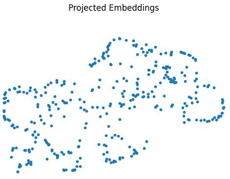
Figure 2: UMAP 2D Projection of 348 dimensional word embedding
Although the resulting 2D visualizations might sometimes appear odd, it’s important to remember that they represent a highly complex, high-dimensional space compressed into just two dimensions. Bringing our thinking into a geometric setting helps us better understand what’s happening behind the scenes in retrieval systems. It’s like looking at a map: the 2D representation helps us navigate the intricate terrain of high-dimensional embeddings.
Relevancy and Distraction in Retrieval
What is the main considerations for an Infomration Retrieval System? The information that you retrieve is either going to be relevant or a distraction. Figure 3 shows a visualisation for an in-scope query and the retrieved chunks of information using a vector similarity matrix. The embedding for the query is shown by the red ‘X’ and the retrieved embeddings are shown by the green ‘O’.
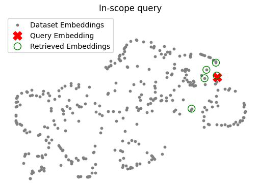
Figure 3: UMAP Projection of an In scope query
One might notice that the points on the 2D visualization don’t always align perfectly with their nearest neighbors in the original high-dimensional space. This discrepancy arises because the embedding model used lacks specific knowledge of the tasks or queries it’s being applied to. Thus, retrieving information for specific tasks can be more challenging when relying solely on a general representation.
Understanding Distractors
In the realm of information retrieval, distractors refer to the irrelevant information retrieved that doesn’t pertain to the query. Diagnosing and debugging these distractors is a significant challenge for users, engineers, and developers alike.
To visualise this, imagine the 2D embedding space as a cloud. A vector representing a query that lands outside this cloud will, by definition, find its nearest neighbors scattered throughout different points in the cloud. This geometrical intuition highlights why totally irrelevant queries can yield a wide array of retrieved information, as designed by the RAG system.
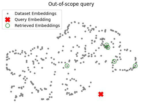
Figure 4: UMAP 2D Projection of an Out of Scope query
In summary, while simple vector searches provide a foundational approach to retrieval, advanced techniques like UMAP offer deeper insights into embedding spaces, helping us understand and improve the relevancy of retrieved information. By visualising and analysing these high-dimensional spaces, we can better navigate the complexities of retrieval-augmented generation systems, ultimately enhancing their effectiveness and reliability. Stay tuned for further exploration into advanced retrieval methods in the upcoming sections.
Improving Retrieval
Information retrieval has long been a crucial subfield of natural language processing (NLP), with numerous approaches developed to enhance the relevancy of query results. The advent of large language models (LLMs) has introduced powerful tools to augment and refine the queries sent to vector databases, significantly improving the quality of the results. In this section, we’ll explore two main types of query expansion: expansion with generated answers and query expansion with multiple queries.
Query Expansion with Example Answers
A novel approach to query expansion involves using LLMs to generate hypothetical or imagined responses to the initial query. This method leverages the model’s ability to create contextually rich content, which can then be used to improve the retrieval process. For full details please refer to the original paper.

Figure 5: Query Expansion using Example Answers
How It Works:
- Generate a Response: Take the original query and prompt the LLM to generate a hypothetical answer. For example, you might use a prompt like: “You are an expert helpful financial research assistant. Provide an example answer to the given question, that might be found in a document like an annual report.”
- Concatenate and Query: Combine the original query with the generated response and use this expanded query to search the vector database.
- Retrieve Results: Perform the retrieval as usual, but with the enhanced query.
Please see below a code snippet to help you expand queries in your projects:
def augment_query_generated(query, model="gpt-3.5-turbo"):
    messages = [
        {
            "role": "system",
            "content": "You are a helpful expert financial research assistant. Provide an example answer to the given question, that might be found in a document like an annual report. "
        },
        {"role": "user", "content": query}
    ]

    response = openai_client.chat.completions.create(
        model=model,
        messages=messages,
    )
    content = response.choices[0].message.content
    return content

original_query = "Was there significant turnover in the executive team?"
hypothetical_answer = augment_query_generated(original_query)

joint_query = f"{original_query} {hypothetical_answer}"
print(word_wrap(joint_query))
Outputs the following expanded query: Was there significant turnover in the executive team? Over the past fiscal year, there have been no significant turnovers within the executive team. The leadership continuity has provided stability and consistency in driving our strategic initiatives forward and achieving our corporate objectives.
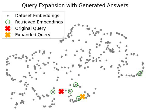
Figure 6: UMAP 2D Projection of Query Expansion with Example/Generated Answers
The figure above illustrates this process: the red X represents the original query, while the orange X signifies the query with the hallucinated response (i.e. the expanded query). The geometrical proximity of the expanded query to the relevant information highlights why this method can extract more contextually appropriate results. The key takeaway from the figure below is that providing an expanded query with additional details about the desired format of the retrieved information can significantly alter the embedding from the original query to the expanded one.
In summary, by using an LLM to generate a plausible answer to the query, you can provide additional relevant context, which enhances the retrieval process. This method allows for the retrieval of more nuanced and contextually relevant results.
Query Expansion with Multiple Queries
Another effective method of query expansion involves generating multiple related queries using an LLM. This approach diversifies the search and increases the likelihood of retrieving comprehensive information relevant to the original query.

Figure 7: Query Expansion with Multiple Queries
How It Works:
- Generate Additional Queries: Prompt the LLM to suggest additional related questions. For instance: “You are a helpful expert financial research assistant. Your users are asking questions about an annual report. Suggest up to five additional related questions to help them find the information they need, for the provided question. Suggest only short questions without compound sentences. Suggest a variety of questions that cover different aspects of the topic. Make sure they are complete questions, and that they are related to the original question. Output one question per line. Do not number the questions.”
- Retrieve Results: Use the original query and the additional queries to retrieve results from the vector database.
- Aggregate and Process: Send all retrieved responses to the LLM for further processing.
def augment_multiple_query(query, model="gpt-3.5-turbo"):
    messages = [
        {
            "role": "system",
            "content": "You are a helpful expert financial research assistant. Your users are asking questions about an annual report. "
            "Suggest up to five additional related questions to help them find the information they need, for the provided question. "
            "Suggest only short questions without compound sentences. Suggest a variety of questions that cover different aspects of the topic."
            "Make sure they are complete questions, and that they are related to the original question."
            "Output one question per line. Do not number the questions."
        },
        {"role": "user", "content": query}
    ]

    response = openai_client.chat.completions.create(
        model=model,
        messages=messages,
    )
    content = response.choices[0].message.content
    content = content.split("\n")
    return content
The figure below illustrates this process: the red X represents the original query, while the orange X’s represent the additional queries. This expansion helps ensure that more relevant information is retrieved, covering various aspects of the original query.
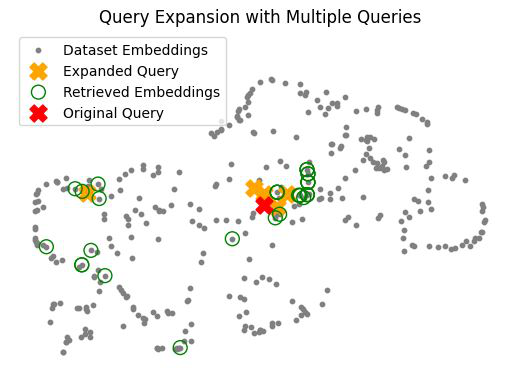
Figure 8: UMAP 2D Projection of Query Expansion with Multiple Queries
Considerations
- Prompt Engineering: Crafting effective prompts is crucial as they become more complex and lengthy.
- Redundancy: Multiple queries might retrieve overlapping information chunks from your vector database. It’s essential to manage and filter these to avoid redundancy.
In summary, query expansion techniques, whether through generated answers or multiple related queries, significantly improve the effectiveness of retrieval-augmented generation systems. By leveraging the capabilities of LLMs, we can refine our search queries, leading to more accurate and contextually relevant results.
However, a big question remains… How can we rank the quality of information retrieved by our system? To ensure that the retrieved results are relevant, scoring mechanisms can be implemented. Each retrieved chunk can be evaluated based on its relevancy to the original query, enhancing the overall precision of the retrieval process.
Cross-Encoder Re-Ranking
One of the key challenges in information retrieval is assessing the relevancy of retrieved results based on the query inputted to the system. Cross-encoder re-ranking addresses this challenge by scoring the relevancy of retrieved results and reordering them to prioritize the most relevant ones.
How it Works
- Querying the Vector Database: Initially, the system queries the vector database and retrieves a set of results.
- Requesting Additional Information: Rather than requesting only a few relevant pieces of information, request additional embeddings as irrelevant ones will later be discarded.
- Re-ranking: The retrieved results are re-ranked based on their relevancy to the original query. The most relevant results are given higher ranks.
- Selection: Finally, the top-ranking results are selected to be inputted to the LLM as context.
Obtain a “Long Tail” of results
We want to obtain more retrieved embeddings from our VectorDB, for example we may consider retrieving 10-15+ chunks rather than the typical 3-5. This means that we will have a “longer tail” of possibly useful results. Once we have retrieved out long tail of results, we need to identify which chunks are actually most relevant to our query, rather than just being the nearest neighbours in embedding space. The way we do this is by using a Cross-encoder to Re-rank the long tail of results.
Cross-Encoders
Unlike bi-encoders, which process sequences separately, cross-encoders process two input sequences together as a single input. This allows the model to directly compare and contrast the inputs, leading to a more integrated and nuanced understanding of their relationship.
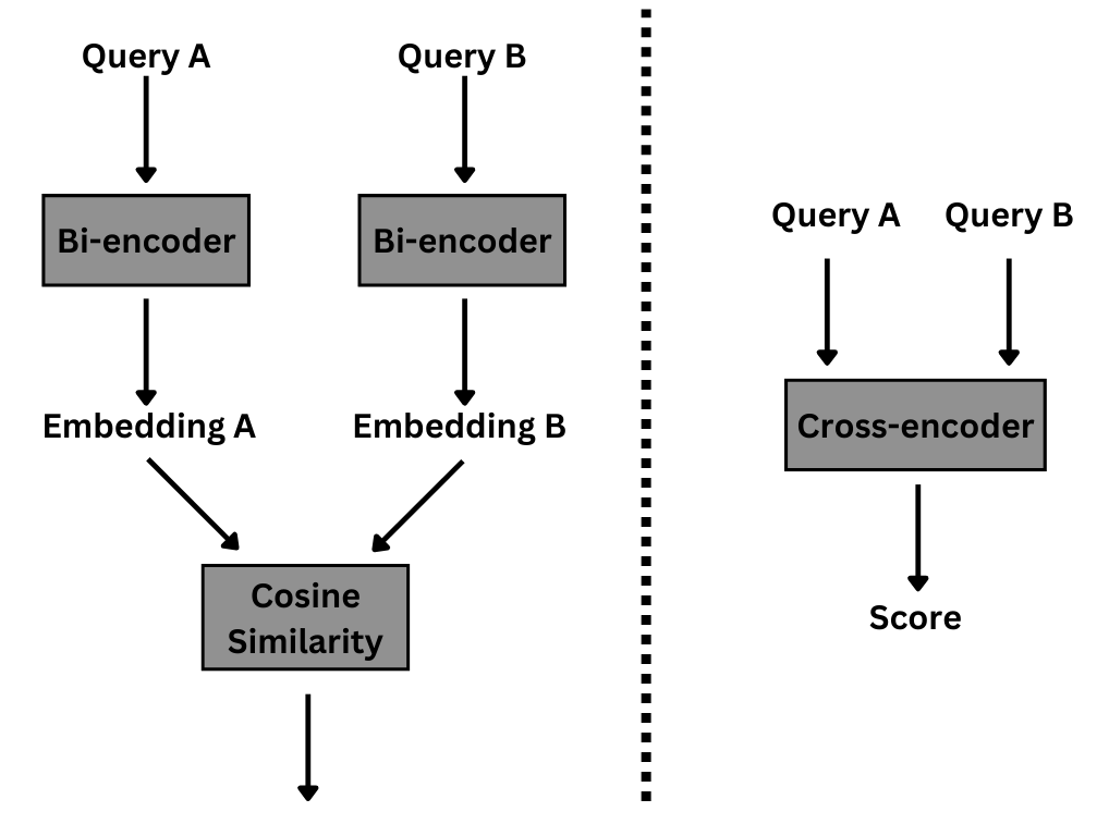
Figure 9: Bi-encoder vs. Cross-encoder to generate
Re-ranking with Query Expansion
Integrating query expansion with cross-encoder re-ranking enhances the retrieval process.
Firstly, use one of the query expansion techniques already mentioned in this blog post such as using generated answers or multiple prompts.
query = "What has been the investment in research and development?"
results = chroma_collection.query(query_texts=query, n_results=10, include=['documents', 'embeddings'])

retrieved_documents = results['documents'][0]

for document in results['documents'][0]:
    print(word_wrap(document))
    print('')
Then, use a Cross-Encoder to predict scores for each retrieved chunk of information with the query. Re-rank the chunks based on the scores given and discard any chunks which are not contextually relevant to the prompt.
from sentence_transformers import CrossEncoder
cross_encoder = CrossEncoder('cross-encoder/ms-marco-MiniLM-L-6-v2')

pairs = [[query, doc] for doc in retrieved_documents]
scores = cross_encoder.predict(pairs)

new_ordering = []
for o in np.argsort(scores)[::-1]:
    new_ordering.append(o+1)
The table below has been produced to display the original order, cross-encoder scores and new order (based on the cross encoder scores) for the retrieved information. Various thresholds may be considered for discarding irrelevant information such as using K-most relevant chunks, or any chunks with a cross-encoder score greater than a threshold (i.e greater than 0).
| Original Ordering | Cross-Encoder Scores | New Ordering |
|---|---|---|
| 1 | 0.98693466 | 2 |
| 2 | 2.644579 | 1 |
| 3 | -0.26802942 | 3 |
| 4 | -10.73159 | 7 |
| 5 | -7.7066045 | 6 |
| 6 | -5.6469955 | 9 |
| 7 | -4.297035 | 10 |
| 8 | -10.933233 | 5 |
| 9 | -7.0384283 | 4 |
| 10 | -7.3246956 | 8 |
By combining cross-encoder re-ranking with query expansion, retrieval-augmented generation systems can effectively extract and present the most contextually relevant information to the final LLM. This integrated approach maximizes the utility of retrieved results, particularly in scenarios involving extensive datasets or complex queries. Stay tuned for more insights into advanced retrieval methods that utilise user feedback to improve retrieval quality.
Embedding Adaptors
Another key method for enhancing the quality of retrieval systems is through the use of Embedding Adaptors. By leveraging user feedback on the relevancy of retrieved results, we can significantly enhance the performance of retrieval systems. Let’s delve into how this process works and how you can implement it using PyTorch.
An Embedding Adaptor is a transformation that is applied to your word embedding for your query. The main idea behind this is that you apply this transformation to your query embedding just after it is outputted from the embedding model, and before you execute your similarity search between your query and Vector Database as shown in the pipeline diagram below.

Figure 10: Embedding Adaptor
Preparing the dataset
The core idea is to use user feedback to train your Embedding Adaptor to encourage the system to retrieve information that is more contextually relevant to your use case. Here is an outline of the process:
- Data Collection: Start by gathering a set of queries for your system. You could generate these using a LLM to get started.
- Retrieve Initial Results: Use your vector database to fetch results for each query.
- Evaluate Results: Utilize a thumbs-up or thumbs-down system (+1 or -1) to rate the relevance of each result. LLMs can be employed to synthesize this data.
- Relevant results are rated as +1.
- Irrelevant results are rated as -1.
- Prepare Data Arrays:
- Adapter Query Embeddings: The queries used in your system.
- Adapter Document Embeddings: The chunks retrieved from your vector database.
- Adapter Labels: The thumbs-up or thumbs-down ratings.
- Transform and Organize Data: Convert the data into PyTorch tensors and place them into a Torch dataset object.
Building the Embedding Adaptor Model
A good baseline model is essentially just a matrix the same dimensions as your query embedding. You can initialise this with random numbers and we will update the values in a training loop.
The model architecture is straightforward yet powerful:
- Inputs: Query embedding, document embedding, and adaptor matrix.
- Computation:
- Update the query embedding by multiplying it with the adaptor matrix.
- Calculate the cosine similarity between the updated query embedding and the document embedding.
See the PyTorch code snippet below to see how simple it is to implement this:
def embedding_adaptor_model(query_embedding, document_embedding, adaptor_matrix):
    updated_query_embedding = torch.matmul(adaptor_matrix, query_embedding)
    return torch.cosine_similarity(updated_query_embedding, document_embedding, dim=0)

# Initialize the adaptor matrix
mat_size = len(adapter_query_embeddings[0])
adapter_matrix = torch.randn(mat_size, mat_size, requires_grad=True)
Loss Function and Training
- Loss Function: Use Mean Squared Error (MSELoss) to measure the difference between the model’s predictions and the actual labels.
- Initialisation: Begin by using the shape of your query embedding with random values for the Embedding Adaptor Matrix.
- Training Efficiency: Training is fast as the model is basically a single linear layer in a multilayer perceptron or artificial neural network, making it computationally light.
See below the code snippet for calculating the loss in PyTorch:
def mse_loss(query_embedding, document_embedding, adaptor_matrix, label):
    return torch.nn.MSELoss()(embedding_adaptor_model(query_embedding, document_embedding, adaptor_matrix), label)
Now we have all the key components to train our Embedding Adaptor. Here is a simple training loop:
min_loss = float('inf')
best_matrix = None
lr = 0.01

for epoch in tqdm(range(100)):
    for query_embedding, document_embedding, label in dataset:
        loss = mse_loss(query_embedding, document_embedding, adapter_matrix, label)

        if loss < min_loss:
            min_loss = loss
            best_matrix = adapter_matrix.clone().detach().numpy()

        loss.backward()
        with torch.no_grad():
            adapter_matrix -= lr * adapter_matrix.grad
            adapter_matrix.grad.zero_()
Impact of the Embedding Adaptor
The adaptor matrix plays a crucial role in refining the query vector emphasising the dimensions with high importance to the task and minimising the dimensions with low importance to the task based on user feedback. How can you visualise the impact of the Embedding Adaptor?
- Transformation Example: Create a test vector of with all values set to 1 and multiply this by the trained Embedding Adaptor Matrix and you can observed how the dimensions of the vector have been stretched and squeezed.
- Dimensional Emphasis: The transformation that the Embedding Adaptor Matrix applies emphasizes the dimensions that are most relevant to the query and diminishes those that are less relevant (based on user feedback), thereby tailoring the feature vectors to improve retrieval accuracy.
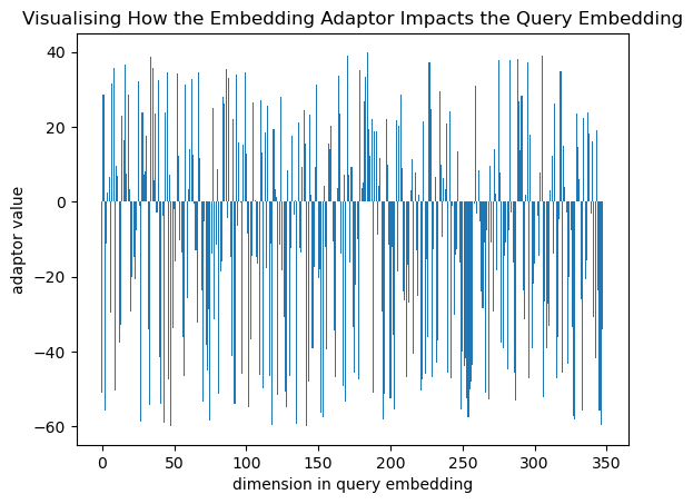
Figure 11: Embedding Adaptor Matrix Visualised
By implementing embedding adaptors, you can create a more responsive and accurate retrieval system that learns and adapts based on user feedback. This method not only enhances the relevance of retrieved results but also ensures that your system evolves continuously to meet user needs. As shown in the figure below, the original query embeddings are more scattered and the adapted queries are more concentrated. This is indicative that the adaptive query embeddings have clustered nearby areas of the vector database that are more relevant. This demonstrates how embedding adaptors are simple but powerful techniques for customizing query embeddings for a particular use case based and can utilise feedback from your application.
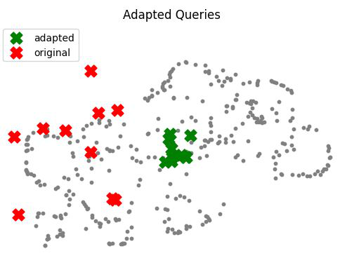
Figure 12: Embedding Adaptor Matrix Visualised
Incorporate these steps and insights into your AI projects to witness a significant boost in performance and user satisfaction.
Conclusion
In this blog post we have covered the following:
- How to compute UMAP projections to visualise your Vector Database in 2 dimensions
- Query expansion using generated answers
- Query expansion with multiple prompts
- Cross-encoder re-ranking
- Embedding Adaptors
This has been a summary of a course I took and I have pushed the code to my GitHub if you would like to explore it further!
